A Tutorial Introduction
We will begin by a quick tutorial on Knet, going over the essential tools for defining, training, and evaluating real machine learning models in 10 short lessons. The examples cover linear regression, softmax classification, multilayer perceptrons, convolutional and recurrent neural networks. We will use these models to predict housing prices in Boston, recognize handwritten digits, and teach the computer to write like Shakespeare!
The goal is to get you to the point where you can create your own models and apply machine learning to your own problems as quickly as possible. So some of the details and exceptions will be skipped for now. No prior knowledge of machine learning or Julia is necessary, but general programming experience will be assumed. It would be best if you follow along with the examples on your computer. Before we get started please complete the installation instructions if you have not done so already.
1. Functions and models
See also
@knet, function, compile, forw, get, :colon
In this section, we will create our first Knet model, and learn how to
make predictions. To start using Knet, type using Knet at the
Julia prompt:
julia> using Knet
...
In Knet, a machine learning model is defined using a special function
syntax with the @knet macro. It may be helpful at this point to
review the Julia function syntax as the Knet syntax is based on it.
The following example defines a @knet function for a simple linear
regression model with 13 inputs and a single output. You can type this
definition at the Julia prompt, or you can copy and paste it into a
file which can be loaded into Julia using include("filename"):
@knet function linreg(x)
    w = par(dims=(1,13), init=Gaussian(0,0.1))
    b = par(dims=(1,1),  init=Constant(0))
    return w * x .+ b
end
In this definition:
@knetindicates thatlinregis a Knet function, and not a regular Julia function or variable.xis the only input argument. We will use a(13,1)column vector for this example.wandbare model parameters as indicated by theparconstructor.dimsandinitare keyword arguments topar.dimsgives the dimensions of the parameter. Julia stores arrays in column-major order, i.e.(1,13)specifies 1 row and 13 columns.initdescribes how the parameter should be initialized. It can be a user supplied Julia array or one of the supported array fillers as in this example.- The final
returnstatement specifies the output of the Knet function. - The
*denotes matrix product and.+denotes elementwise broadcasting addition. - Broadcasting operations like
.+can act on arrays with different sizes, such as adding a vector to each column of a matrix. They expand singleton dimensions in array arguments to match the corresponding dimension in the other array without using extra memory, and apply the operation elementwise. - Unlike regular Julia functions, only a restricted set of
operators such as
*and.+, and statement types such as assignments and returns can be used in a @knet function definition.
In order to turn linreg into a machine learning model that can be
trained with examples and used for predictions, we need to compile it:
julia> f1 = compile(:linreg)        # The colon before linreg is required
...
To test our model let’s give it some input initialized with random numbers:
julia> x1 = randn(13,1)
13x1 Array{Float64,2}:
 -0.556027
 -0.444383
 ...
To obtain the prediction of model f1 on input x1 we use the
forw function, which basically calculates w * x1 .+ b:
julia> forw(f1,x1)
1x1 Array{Float64,2}:
 -0.710651
We can query the model and see its parameters using get:
julia> get(f1,:w)           # The colon before w is required
1x13 Array{Float64,2}:
 0.149138  0.0367563  ... -0.433747  0.0569829

julia> get(f1,:b)
1x1 Array{Float64,2}:
 0.0
We can also look at the input with get(f1,:x), reexamine the output
using the special :return symbol with get(f1,:return). In fact
using get, we can confirm that our model gives us the same answer
as an equivalent Julia expression:
julia> get(f1,:w) * get(f1,:x) .+ get(f1,:b)
1x1 Array{Float64,2}:
 -0.710651 DBG
You can see the internals of the compiled model looking at f1. It
consists of 5 low level operations:
julia> f1
1 Knet.Input() name=>x,dims=>(13,1),norm=>3.84375,...
2 Knet.Par() name=>w,dims=>(1,13),norm=>0.529962,...
3 Knet.Par() name=>b,dims=>(1,1),norm=>0 ,...
4 Knet.Dot(2,1) name=>##tmp#7298,args=>(w,x),dims=>(1,1),norm=>0.710651,...
5 Knet.Add(4,3) name=>return,args=>(##tmp#7298,b),dims=>(1,1),norm=>0.710651,...
You may have noticed the colons before Knet variable names like
:linreg, :w, :x, :b, etc. Any variable introduced in
a @knet macro is not a regular Julia variable so its name needs to be
escaped using the colon character in ordinary Julia code. In
contrast, f1 and x1 are ordinary Julia variables.
In this section, we have seen how to create a Knet model by compiling
a @knet function, how to perform a prediction given an input using
forw, and how to take a look at model parameters using get.
Next we will see how to train models.
2. Training a model
See also
back, update!, setp, lr, quadloss
OK, so we can define functions using Knet but why should we bother? The thing that makes a Knet function different from an ordinary function is that Knet functions are differentiable programs. This means that for a given input not only can they compute an output, but they can also compute which way their parameters should be modified to approach some desired output. If we have some input-output data that comes from an unknown function, we can train a Knet model to look like this unknown function by manipulating its parameters.
We will use the Housing dataset from the UCI Machine Learning
Repository to train our linreg model. The dataset has housing
related information for 506 neighborhoods in Boston from 1978. Each
neighborhood has 14 attributes, the goal is to use the first 13, such
as average number of rooms per house, or distance to employment
centers, to predict the 14’th attribute: median dollar value of the
houses. Here are the first 3 entries:
0.00632  18.00   2.310  0  0.5380  6.5750  65.20  4.0900   1  296.0  15.30 396.90   4.98  24.00
0.02731   0.00   7.070  0  0.4690  6.4210  78.90  4.9671   2  242.0  17.80 396.90   9.14  21.60
0.02729   0.00   7.070  0  0.4690  7.1850  61.10  4.9671   2  242.0  17.80 392.83   4.03  34.70
...
Let’s download the dataset and use readdlm to turn
it into a Julia array.
julia> url = "https://archive.ics.uci.edu/ml/machine-learning-databases/housing/housing.data";
julia> file = Pkg.dir("Knet/data/housing.data");
julia> download(url, file)
  ...
julia> data = readdlm(file)'  # Don't forget the final apostrophe to transpose data
14x506 Array{Float64,2}:
   0.00632    0.02731    0.02729 ...   0.06076    0.10959    0.04741
  18.0        0.0        0.0     ...   0.0        0.0        0.0
  ...
The resulting data matrix should have 506 columns representing
neighborhoods, and 14 rows representing the attributes. The last
attribute is the median house price to be predicted, so let’s separate
it:
julia> x = data[1:13,:]
13x506 Array{Float64,2}:...
julia> y = data[14,:]
1x506 Array{Float64,2}:...
Here we are using Julia’s array indexing notation to split the
data array into input x and output y. Inside the square
brackets 1:13 means grab the rows 1 through 13, and the :
character by itself means grab all the columns.
You may have noticed that the input attributes have very different ranges. It is usually a good idea to normalize them by subtracting the mean and dividing by the standard deviation:
julia> x = (x .- mean(x,2)) ./ std(x,2);
The mean() and std() functions compute the mean and
standard deviation of x. Their optional second argument gives the
dimensions to sum over, so mean(x) gives us the mean of the whole
array, mean(x,1) gives the mean of each column, and mean(x,2)
gives us the mean of each row.
It is also a good idea to split our dataset into training and test subsets so we can estimate how well our model will do on unseen data.
julia> n = size(x,2);
julia> r = randperm(n);
julia> xtrn=x[:,r[1:400]];
julia> ytrn=y[:,r[1:400]];
julia> xtst=x[:,r[401:end]];
julia> ytst=y[:,r[401:end]];
n is set to the number of instances (columns) and r is set to
randperm(n) which gives a random permutation of
integers \(1\ldots n\). The first 400 indices in r will be
used for training, and the last 106 for testing.
Let’s see how well our randomly initialized model does before training:
julia> ypred = forw(f1, xtst)
1x10⁶ Array{Float64,2}:...
julia> quadloss(ypred, ytst)
307.9336...
The quadratic loss function quadloss()
computes \((1/2n) \sum (\hat{y} - y)^2\), i.e. half of the mean
squared difference between a predicted answer \(\hat{y}\) and the
desired answer \(y\). Given that \(y\) values range from 5 to
50, an RMSD of \(\sqrt{2\times 307.9}=24.8\) is a pretty bad
score.
We would like to minimize this loss which should get the predicted
answers closer to the desired answers. To do this we first compute
the loss gradient for the parameters of f1 – this is the direction
in parameter space that maximally increases the loss. Then we move
the parameters in the opposite direction. Here is a simple function
that performs these steps:
function train(f, x, y)
    for i=1:size(x,2)
        forw(f, x[:,i])
        back(f, y[:,i], quadloss)
        update!(f)
    end
end
- The
forloop grabs training instances one by one. forwcomputes the prediction for the i’th instance. This is required for the next step.backcomputes the loss gradient for each parameter inffor the i’th instance.update!moves each parameter opposite the gradient direction to reduce the loss.
Before training, it is important to set a good learning rate. The
learning rate controls how large the update steps are going to be: too
small and you’d wait for a long time, too large and train may
never converge. The setp() function is used to set
training options like the learning rate. Let’s
set the learning rate to 0.001 and train the model for 100 epochs
(i.e. 100 passes over the dataset):
julia> setp(f1, lr=0.001)
julia> for i=1:100; train(f1, xtrn, ytrn); end
This should take a few seconds, and this time our RMSD should be much better:
julia> ypred = forw(f1, xtst)
1x10⁶ Array{Float64,2}:...
julia> quadloss(ypred,ytst)
11.5989...
julia> sqrt(2*ans)
4.8164...
We can see what the model has learnt looking at the new weights:
julia> get(f1,:w)
1x13 Array{Float64,2}:
 -0.560346  0.924687  0.0446596  ...  -1.89473  1.13219  -3.51418 DBG
The two weights with the most negative contributions are 13 and 8. We can find out from UCI that these are:
13. LSTAT: % lower status of the population
 8. DIS: weighted distances to five Boston employment centres
And the two with the most positive contributions are 9 and 6:
9. RAD: index of accessibility to radial highways
6. RM: average number of rooms per dwelling
In this section we saw how to download data, turn it into a Julia
array, normalize and split it into input, output, train, and test
subsets. We wrote a simple training script using forw, back,
and update!, set the learning rate lr using setp, and
evaluated the model using the quadloss loss function. Now, there
are a lot more efficient and elegant ways to perform and analyze a
linear regression as you can find out from any decent statistics text.
However the basic method outlined in this section has the advantage of
being easy to generalize to models that are a lot larger and
complicated.
3. Making models generic
See also
keyword arguments, size inference
Hardcoding the dimensions of parameters in linreg makes it
awfully specific to the Housing dataset. Knet allows keyword
arguments in @knet function definitions to get around this problem:
@knet function linreg2(x; inputs=13, outputs=1)
    w = par(dims=(outputs,inputs), init=Gaussian(0,0.1))
    b = par(dims=(outputs,1), init=Constant(0))
    return w * x .+ b
end
Now we can use this model for another dataset that has, for example,
784 inputs and 10 outputs by passing these keyword arguments to
compile:
julia> f2 = compile(:linreg2, inputs=784, outputs=10);
Knet functions borrow the syntax for keyword arguments from Julia,
and we will be using them in many contexts, so a brief aside is in
order: Keyword arguments are identified by name instead of position,
and they can be passed in any order (or not passed at all) following
regular (positional) arguments. In fact we have already seen
examples: dims and init are keyword arguments for par
(which has no regular arguments). Functions with keyword arguments
are defined using a semicolon in the signature, e.g. function
pool(x; window=2, padding=0). The semicolon is optional when the
function is called, e.g. both pool(x, window=5) or pool(x;
window=5) work. Unspecified keyword arguments take their default
values specified in the function definition. Extra keyword arguments
can be collected using three dots in the function definition:
function pool(x; window=2, padding=0, o...), and passed in
function calls: pool(x; o...).
In addition to keyword arguments to make models more generic, Knet implements size inference: Any dimension that relies on the input size can be left as 0, which tells Knet to infer that dimension when the first input is received. Leaving input dependent dimensions as 0, and using a keyword argument to determine output size we arrive at a fully generic version of linreg:
@knet function linreg3(x; out=1)
    w = par(dims=(out,0), init=Gaussian(0,0.1))
    b = par(dims=(out,1), init=Constant(0))
    return w * x .+ b
end
In this section, we have seen how to make @knet functions more generic using keyword arguments and size inference. This will especially come in handy when we are using them as new operators as described next.
4. Defining new operators
See also
@knet function as operator, soft
The key to controlling complexity in computer languages is abstraction. Abstraction is the ability to name compound structures built from primitive parts, so they too can be used as primitives. In Knet we do this by using @knet functions not just as models, but as new operators inside other @knet functions.
To illustrate this, we will implement a softmax classification model. Softmax classification is basically linear regression with multiple outputs followed by normalization. Here is how we can define it in Knet:
@knet function softmax(x; out=10)
    z = linreg3(x; out=out)
    return soft(z)
end
The softmax model basically computes soft(w * x .+ b) with
trainable parameters w and b by calling linreg3 we defined
in the previous section. The out keyword parameter determines the
number of outputs and is passed from softmax to linreg3
unchanged. The number of inputs is left unspecified and is inferred
when the first input is received. The soft operator normalizes
its argument by exponentiating its elements and dividing each by their
sum.
In this section we saw an example of using a @knet function as a new operator. Using the power of abstraction, not only can we avoid repetition and shorten the amount of code for larger models, we make the definitions a lot more readable and configurable, and gain a bunch of reusable operators to boot. To see some example reusable operators take a look at the Knet compound operators table and see their definitions in kfun.jl.
5. Training with minibatches
See also
minibatch, softloss, zeroone
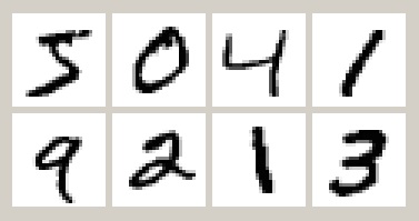
We will use the softmax model to classify hand-written digits from the MNIST dataset. Here are the first 8 images from MNIST, the goal is to look at the pixels and classify each image as one of the digits 0-9:
The following loads the MNIST data:
julia> include(Pkg.dir("Knet/examples/mnist.jl"))
INFO: Loading MNIST...
Once loaded, the data is available as multi-dimensional Julia arrays:
julia> MNIST.xtrn
28x28x1x60000 Array{Float32,4}:...
julia> MNIST.ytrn
10x60000 Array{Float32,2}:...
julia> MNIST.xtst
28x28x1x10000 Array{Float32,4}:...
julia> MNIST.ytst
10x10000 Array{Float32,2}:...
We have 60000 training and 10000 testing examples. Each input x is a
28x28x1 array representing one image, where the first two numbers
represent the width and height in pixels, the third number is the
number of channels (which is 1 for grayscale images, 3 for RGB
images). The softmax model will treat each image as a 28*28*1=784
dimensional vector. The pixel values have been normalized to
\([0,1]\). Each output y is a ten-dimensional one-hot vector (a
vector that has a single non-zero component) indicating the correct
class (0-9) for a given image.
This is a much larger dataset than Housing. For computational
efficiency, it is not advisable to use these examples one at a time
during training like we did before. We will split the data into
groups of 100 examples called minibatches, and pass data to
forw and back one minibatch at a time instead of one instance
at a time. On my laptop, one epoch of training softmax on MNIST takes
about 0.34 seconds with a minibatch size of 100, 1.67 seconds with a
minibatch size of 10, and 10.5 seconds if we do not use minibatches.
Knet provides a small minibatch function to split the data:
function minibatch(x, y, batchsize)
    data = Any[]
    for i=1:batchsize:ccount(x)
        j=min(i+batchsize-1,ccount(x))
        push!(data, (cget(x,i:j), cget(y,i:j)))
    end
    return data
end
minibatch takes batchsize columns of x and y at a
time, pairs them up and pushes them into a data array. It works
for arrays of any dimensionality, treating the last dimension as
“columns”. Note that this type of minibatching is fine for small
datasets, but it requires holding two copies of the data in memory.
For problems with a large amount of data you may want to use
subarrays or iterables.
Here is minibatch in action:
julia> batchsize=100;
julia> trn = minibatch(MNIST.xtrn, MNIST.ytrn, batchsize)
600-element Array{Any,1}:...
julia> tst = minibatch(MNIST.xtst, MNIST.ytst, batchsize)
100-element Array{Any,1}:...
Each element of trn and tst is an x, y pair that contains 100
examples:
julia> trn[1]
(28x28x1x100 Array{Float32,4}: ...,
 10x100 Array{Float32,2}: ...)
Here are some simple train and test functions that use this type of minibatched data. Note that they take the loss function as a third argument and iterate through the x,y pairs (minibatches) in data:
function train(f, data, loss)
    for (x,y) in data
        forw(f, x)
        back(f, y, loss)
        update!(f)
    end
end

function test(f, data, loss)
    sumloss = numloss = 0
    for (x,ygold) in data
        ypred = forw(f, x)
        sumloss += loss(ypred, ygold)
        numloss += 1
    end
    return sumloss / numloss
end
Before training, we compile the model and set the learning rate to
0.2, which works well for this example. We use two new loss
functions: softloss computes the cross entropy loss,
\(E(p\log\hat{p})\), commonly used for training classification
models and zeroone computes the zero-one loss which is the
proportion of predictions that were wrong. I got 7.66% test error
after 40 epochs of training. Your results may be slightly different
on different machines, or different runs on the same machine because
of random initialization.
julia> model = compile(:softmax);
julia> setp(model; lr=0.2);
julia> for epoch=1:40; train(model, trn, softloss); end
julia> test(model, tst, zeroone)
0.0766...
In this section we saw how splitting the training data into
minibatches can speed up training. We trained our first
classification model on MNIST and used two new loss functions:
softloss and zeroone.
6. MLP
7. Convnet
Deprecated
See also
@knet as op, kwargs for @knet functions, function options (f=:relu). splat. lenet example, fast enough on cpu?
To illustrate this, we will use the LeNet convolutional neural network model designed to recognize handwritten digits. Here is the LeNet model defined using only the primitive operators of Knet:
@knet function lenet1(x)    # dims=(28,28,1,N)
    w1 = par(init=Xavier(),   dims=(5,5,1,20))
    c1 = conv(w1,x)         # dims=(24,24,20,N)
    b1 = par(init=Constant(0),dims=(1,1,20,1))
    a1 = add(b1,c1)
    r1 = relu(a1)
    p1 = pool(r1; window=2) # dims=(12,12,20,N)

    w2 = par(init=Xavier(),   dims=(5,5,20,50))
    c2 = conv(w2,p1)        # dims=(8,8,50,N)
    b2 = par(init=Constant(0),dims=(1,1,50,1))
    a2 = add(b2,c2)
    r2 = relu(a2)
    p2 = pool(r2; window=2) # dims=(4,4,50,N)

    w3 = par(init=Xavier(),   dims=(500,800))
    d3 = dot(w3,p2)         # dims=(500,N)
    b3 = par(init=Constant(0),dims=(500,1))
    a3 = add(b3,d3)
    r3 = relu(a3)

    w4 = par(init=Xavier(),   dims=(10,500))
    d4 = dot(w4,r3)         # dims=(10,N)
    b4 = par(init=Constant(0),dims=(10,1))
    a4 = add(b4,d4)
    return soft(a4)         # dims=(10,N)
end
Don’t worry about the details of the model if you don’t know much about neural nets. At 22 lines long, this model looks a lot more complicated than our linear regression model. Compared to state of the art image processing models however, it is still tiny. You would not want to code a state-of-the-art model like GoogLeNet using these primitives.
If you are familiar with neural nets, and peruse the Knet primitives table, you can see that the model has two convolution-pooling layers (commonly used in image processing), a fully connected relu layer and a final softmax output layer (I separated them by blank lines to help). Wouldn’t it be nice to say just that:
@knet function lenet2(x)
    a = conv_pool_layer(x)
    b = conv_pool_layer(a)
    c = relu_layer(b)
    return softmax_layer(c)
end
lenet2 is a lot more readable than lenet1. But before we can
use this definition, we have to solve two problems:
conv_pool_layeretc. are not primitive operators, we need a way to add them to Knet.- Each layer has some attributes, like
initanddims, that we need to be able to configure.
Knet solves the first problem by allowing @knet functions to be used
as operators as well as models. For example, we can define
conv_pool_layer as an operator with:
@knet function conv_pool_layer(x)
    w = par(init=Xavier(), dims=(5,5,1,20))
    c = conv(w,x)
    b = par(init=Constant(0), dims=(1,1,20,1))
    a = add(b,c)
    r = relu(a)
    return pool(r; window=2)
end
With this definition, the the first a = conv_pool_layer(x)
operation in lenet2 will work exactly as we want, but not the
second (it has different convolution dimensions).
This brings us to the second problem, layer configuration. It would
be nice not to hard-code numbers like (5,5,1,20) in the definition
of a new operation like conv_pool_layer. Making these numbers
configurable would make such operations more reusable across models.
Even within the same model, you may want to use the same layer type in
more than one configuration. For example in lenet2 there is no
way to distinguish the two conv_pool_layer operations, but looking
at lenet1 we clearly want them to do different things.
Knet solves the layer configuration problem using keyword
arguments. Knet functions borrow the keyword argument syntax from
Julia, and we will be using them in many contexts, so a brief aside is
in order: Keyword arguments are identified by name instead of
position, and they can be passed in any order (or not passed at all)
following regular (positional) arguments. In fact we have already
seen examples: dims and init are keyword arguments for par
(which has no regular arguments) and window is a keyword argument
for pool. Functions with keyword arguments are defined using a
semicolon in the signature, e.g. function pool(x; window=2,
padding=0). The semicolon is optional when the function is called,
e.g. both pool(x, window=5) or pool(x; window=5) work.
Unspecified keyword arguments take their default values specified in
the function definition. Extra keyword arguments can be collected
using three dots in the function definition: function pool(x;
window=2, padding=0, o...), and passed in function calls: pool(x;
o...).
Here is a configurable version of conv_pool_layer using keyword
arguments:
@knet function conv_pool_layer(x; cwindow=0, cinput=0, coutput=0, pwindow=0)
    w = par(init=Xavier(), dims=(cwindow,cwindow,cinput,coutput))
    c = conv(w,x)
    b = par(init=Constant(0), dims=(1,1,coutput,1))
    a = add(b,c)
    r = relu(a)
    return pool(r; window=pwindow)
end
Similarly, we can define relu_layer and softmax_layer with
keyword arguments and make them more reusable. If you did this,
however, you’d notice that we are repeating a lot of code. That is
almost always a bad idea. Why don’t we define a generic_layer
that contains the shared code for all our layers:
@knet function generic_layer(x; f1=:dot, f2=:relu, wdims=(), bdims=(), winit=Xavier(), binit=Constant(0))
    w = par(init=winit, dims=wdims)
    y = f1(w,x)
    b = par(init=binit, dims=bdims)
    z = add(b,y)
    return f2(z)
end
Note that in this example we are not only making initialization
parameters like winit and binit configurable, we are also
making internal operators like relu and dot configurable
(their names need to be escaped with colons when passed as keyword
arguments). This generic layer will allow us to define many layer
types easily:
@knet function conv_pool_layer(x; cwindow=0, cinput=0, coutput=0, pwindow=0)
    y = generic_layer(x; f1=:conv, f2=:relu, wdims=(cwindow,cwindow,cinput,coutput), bdims=(1,1,coutput,1))
    return pool(y; window=pwindow)
end

@knet function relu_layer(x; input=0, output=0)
    return generic_layer(x; f1=:dot, f2=:relu, wdims=(output,input), bdims=(output,1))
end

@knet function softmax_layer(x; input=0, output=0)
    return generic_layer(x; f1=:dot, f2=:soft, wdims=(output,input), bdims=(output,1))
end
Finally we can define a working version of LeNet using 4 lines of code:
@knet function lenet3(x)
    a = conv_pool_layer(x; cwindow=5, cinput=1,  coutput=20, pwindow=2)
    b = conv_pool_layer(a; cwindow=5, cinput=20, coutput=50, pwindow=2)
    c = relu_layer(b; input=800, output=500)
    return softmax_layer(c; input=500, output=10)
end
There are still a lot of hard-coded dimensions in lenet3. Some of
these, like the filter size (5), and the hidden layer size (500) can
be considered part of the model design. We should make them
configurable so the user can experiment with different sized models.
But some, like the number of input channels (1), and the input to the
relu_layer (800) are determined by input size. If we tried to
apply lenet3 to a dataset with different sized images, it would
break. Knet solves this problem using size inference: Any
dimension that relies on the input size can be left as 0, which tells
Knet to infer that dimension when the first input is received.
Leaving input dependent dimensions as 0, and using keyword arguments
to determine model size we arrive at a fully configurable version of
LeNet:
@knet function lenet4(x; cwin1=5, cout1=20, pwin1=2, cwin2=5, cout2=50, pwin2=2, hidden=500, nclass=10)
    a = conv_pool_layer(x; cwindow=cwin1, coutput=cout1, pwindow=pwin1)
    b = conv_pool_layer(a; cwindow=cwin2, coutput=cout2, pwindow=pwin2)
    c = relu_layer(b; output=hidden)
    return softmax_layer(c; output=nclass)
end
To compile an instance of lenet4 with particular dimensions, we
pass keyword arguments to compile:
julia> f = compile(:lenet4; cout1=30, cout2=60, hidden=600)
...
In this section we saw how to use @knet functions as new operators, and configure them using keyword arguments. Using the power of abstraction, not only did we cut the amount of code for the LeNet model in half, we made its definition a lot more readable and configurable, and gained a bunch of reusable operators to boot. I am sure you can think of more clever ways to define LeNet and other complex models using your own set of operators. To see some example reusable operators take a look at the Knet compound operators table and see their definitions in kfun.jl.
8. Conditional Evaluation
See also
if-else, runtime conditions (kwargs for forw), dropout
There are cases where you want to execute parts of a model conditionally, e.g. only during training, or only during some parts of the input in sequence models. Knet supports the use of runtime conditions for this purpose. We will illustrate the use of conditions by implementing a training technique called dropout to improve the generalization power of the LeNet model.
If you keep training the LeNet model on MNIST for about 30 epochs you will observe that the training error drops to zero but the test error hovers around 0.8%:
for epoch=1:100
    train(net, trn, softloss)
    println((epoch, test(net, trn, zeroone), test(net, tst, zeroone)))
end

(1,0.020466666666666505,0.024799999999999996)
(2,0.013649999999999905,0.01820000000000001)
...
(29,0.0,0.008100000000000003)
(30,0.0,0.008000000000000004)
This is called overfitting. The model has memorized the training set, but does not generalize equally well to the test set.
Dropout prevents overfitting by injecting random noise into the model.
Specifically, for each forw call during training, dropout layers
placed between two operations replace a random portion of their input
with zeros, and scale the rest to keep the total output the same.
During testing random noise would degrade performance, so we would
like to turn dropout off. Here is one way to implement this in Knet:
@knet function drop(x; pdrop=0, o...)
    if dropout
        return x .* rnd(init=Bernoulli(1-pdrop, 1/(1-pdrop)))
    else
        return x
    end
end
The keyword argument pdrop specifies the probability of dropping an
input element. The if ... else ... end block causes conditional
evaluation the way one would expect. The variable dropout next to
if is a global condition variable: it is not declared as an argument
to the function. Instead, once a model with a drop operation is
compiled, the call to forw accepts dropout as an optional keyword
argument and passes it down as a global condition:
forw(model, input; dropout=true)
This means every time we call forw, we can change whether dropout
occurs or not. During test time, we would like to stop dropout, so we
can run the model with dropout=false:
forw(model, input; dropout=false)
By default, all unspecified condition variables are false, so we could also omit the condition during test time:
forw(model, input) # dropout=false is assumed
Here is one way to add dropout to the LeNet model:
@knet function lenet5(x; pdrop=0.5, cwin1=5, cout1=20, pwin1=2, cwin2=5, cout2=50, pwin2=2, hidden=500, nclass=10)
    a = conv_pool_layer(x; cwindow=cwin1, coutput=cout1, pwindow=pwin1)
    b = conv_pool_layer(a; cwindow=cwin2, coutput=cout2, pwindow=pwin2)
    bdrop = drop(b; pdrop=pdrop)
    c = relu_layer(bdrop; output=hidden)
    return softmax_layer(c; output=nclass)
end
Whenever the condition variable dropout is true, this will replace
half of the entries in the b array with zeros. We need to modify
our train function to pass the condition to forw:
function train(f, data, loss)
    for (x,y) in data
        forw(f, x; dropout=true)
        back(f, y, loss)
        update!(f)
    end
end
Here is our training script. Note that we reduce the learning rate whenever the test error gets worse, another precaution against overfitting:
lrate = 0.1
decay = 0.9
lasterr = 1.0
net = compile(:lenet5)
setp(net; lr=lrate)

for epoch=1:100
    train(net, trn, softloss)
    trnerr = test(net, trn, zeroone)
    tsterr = test(net, tst, zeroone)
    println((epoch, lrate, trnerr, tsterr))
    if tsterr > lasterr
        lrate = decay*lrate
        setp(net; lr=lrate)
    end
    lasterr = tsterr
end
In 100 epochs, this should converge to about 0.5% error, i.e. reduce the total number of errors on the 10K test set from around 80 to around 50. Congratulations! This is fairly close to the state of the art compared to other benchmark results on the MNIST website:
(1,0.1,0.020749999999999824,0.01960000000000001)
(2,0.1,0.013699999999999895,0.01600000000000001)
...
(99,0.0014780882941434613,0.0003333333333333334,0.005200000000000002)
(100,0.0014780882941434613,0.0003666666666666668,0.005000000000000002)
In this section, we saw how to use the if ... else ... end
construct to perform conditional evaluation in a model, where the
conditions are passed using keyword arguments to forw. We used
this to implement dropout, an effective technique to prevent
overfitting.
9. Recurrent neural networks
See also
read-before-write, simple rnn, lstm
In this section we will see how to implement recurrent neural networks (RNNs) in Knet. A RNN is a class of neural network where connections between units form a directed cycle, which allows them to keep a persistent state (memory) over time. This gives them the ability to process sequences of arbitrary length one element at a time, while keeping track of what happened at previous elements. Contrast this with feed forward nets like LeNet, which have a fixed sized input, output and perform a fixed number of operations. See (Karpathy, 2015) for a nice introduction to RNNs.
To support RNNs, all local variables in Knet functions are static variables, i.e. their values are preserved between calls unless otherwise specified. It turns out this is the only language feature you need to define RNNs. Here is a simple example:
@knet function rnn1(x; hsize=100, xsize=50)
    a = par(init=Xavier(), dims=(hsize, xsize))
    b = par(init=Xavier(), dims=(hsize, hsize))
    c = par(init=Constant(0), dims=(hsize, 1))
    d = a * x .+ b * h .+ c
    h = relu(d)
end
Notice anything strange? The first three lines define three model
parameters. Then the fourth line sets d to a linear combination
of the input x and the hidden state h. But h hasn’t been
defined yet. Exactly! Having read-before-write variables is the only
thing that distinguishes an RNN from feed-forward models like LeNet.
The way Knet handles read-before-write variables is by initializing
them to 0 arrays before any input is processed, then preserving the
values between the calls. Thus during the first call in the above
example, h would start as 0, d would be set to a * x .+ c,
which in turn would cause h to get set to relu(a * x .+ c).
During the second call, this value of h would be remembered and
used, thus making the value of h at time t dependent on
its value at time t-1.
It turns out simple RNNs like rnn1 are not very good at
remembering things for a very long time. There are some techniques to
improve their retention based on better initialization or smarter
updates, but currently the most popular solution is using more
complicated units like LSTMs and GRUs. These units control the
information flow into and out of the unit using gates similar to
digital circuits and can model long term dependencies. See (Colah,
2015) for a good overview of LSTMs.
Defining an LSTM in Knet is almost as concise as writing its mathematical definition:
@knet function lstm(x; fbias=1, o...)
    input  = wbf2(x,h; o..., f=:sigm)
    forget = wbf2(x,h; o..., f=:sigm, binit=Constant(fbias))
    output = wbf2(x,h; o..., f=:sigm)
    newmem = wbf2(x,h; o..., f=:tanh)
    cell = input .* newmem + cell .* forget
    h  = tanh(cell) .* output
    return h
end
The wbf2 operator applies an affine function (linear function +
bias) to its two inputs followed by an activation function (specified
by the f keyword argument). Try to define this operator yourself
as an exercise, (see kfun.jl for the Knet definition).
The LSTM has an input gate, forget gate and an output gate that
control information flow. Each gate depends on the current input
x, and the last output h. The memory value cell is
computed by blending a new value newmem with its old value under
the control of input and forget gates. The output gate
decides how much of the cell is shared with the outside world.
If an input gate element is close to 0, the corresponding element
in the new input x will have little effect on the memory cell. If
a forget gate element is close to 1, the contents of the
corresponding memory cell can be preserved for a long time. Thus the
LSTM has the ability to pay attention to the current input, or
reminisce in the past, and it can learn when to do which based on the
problem.
In this section we introduced simple recurrent neural networks and LSTMs. We saw that having static variables is the only language feature necessary to implement RNNs. Next we will look at how to train them.
10. Training with sequences
(Karpathy, 2015) has lots of fun examples showing how character based language models based on LSTMs are surprisingly adept at generating text in many genres, from Wikipedia articles to C programs. To demonstrate training with sequences, we’ll implement one of these examples and build a model that can write like Shakespeare! After training on “The Complete Works of William Shakespeare” for less than an hour, here is a sample of brilliant writing you can expect from your model:
LUCETTA. Welcome, getzing a knot. There is as I thought you aim
  Cack to Corioli.
MACBETH. So it were timen'd nobility and prayers after God'.
FIRST SOLDIER. O, that, a tailor, cold.
DIANA. Good Master Anne Warwick!
SECOND WARD. Hold, almost proverb as one worth ne'er;
  And do I above thee confer to look his dead;
  I'll know that you are ood'd with memines;
  The name of Cupid wiltwite tears will hold
  As so I fled; and purgut not brightens,
  Their forves and speed as with these terms of Ely
  Whose picture is not dignitories of which,
  Their than disgrace to him she is.
GOBARIND. O Sure, ThisH more.,
  wherein hath he been not their deed of quantity,
  No ere we spoke itation on the tent.
  I will be a thought of base-thief;
  Then tears you ever steal to have you kindness.
  And so, doth not make best in lady,
  Your love was execreed'd fray where Thoman's nature;
  I have bad Tlauphie he should sray and gentle,
First let’s download “The Complete Works of William Shakespeare” from Project Gutenberg:
julia> using Requests
julia> url="http://gutenberg.pglaf.org/1/0/100/100.txt";
julia> text=get(url).data
5589917-element Array{UInt8,1}:...
The text array now has all 5,589,917 characters of “The Complete
Works” in a Julia array. If get does not work, you can download
100.txt by other means and use text=readall("100.txt") on the
local file. We will use one-hot vectors to represent characters, so
let’s map each character to an integer index \(1\ldots n\):
julia> char2int = Dict();
julia> for c in text; get!(char2int, c, 1+length(char2int)); end
julia> nchar = length(char2int)
92
Dict is Julia’s standard associative collection for mapping
arbitrary keys to values. get!(dict,key,default) returns the
value for the given key, storing key=>default in dict if no
mapping for the key is present. Going over the text array we
discover 92 unique characters and map them to integers \(1\ldots
92\).
We will train our RNN to read characters from text in sequence,
and predict the next character after each. The training will go much
faster if we can use the minibatching trick we saw earlier and process
multiple inputs at a time. For that, we split the text array into
batchsize equal length subsequences. Then the first batch has the
first character from each subsequence, second batch contains the
second characters etc. Each minibatch is represented by a nchar x
batchsize matrix with one-hot columns. Here is a function that
implements this type of sequence minibatching:
function seqbatch(seq, dict, batchsize)
    data = Any[]
    T = div(length(seq), batchsize)
    for t=1:T
        d=zeros(Float32, length(dict), batchsize)
        for b=1:batchsize
            c = dict[seq[t + (b-1) * T]]
            d[c,b] = 1
        end
        push!(data, d)
    end
    return data
end
Let’s use it to split text into minibatches of size 128:
julia> batchsize = 128;
julia> data = seqbatch(text, char2int, batchsize)
43671-element Array{Any,1}:...
julia> data[1]
92x128 Array{Float32,2}:...
The data array returned has T=length(text)/batchsize minibatches.
The columns of minibatch data[t] refer to characters t,
t+T, t+2T, ... from text. During training, when
data[t] is the input, data[t+1] will be the desired output.
Now that we have the data ready to go, let’s talk about RNN training.
RNN training is a bit more involved than training feed-forward models.
We still have the prediction, gradient calculation and update steps,
but not all three steps should be performed after every input. Here
is a basic algorithm: Go forward nforw steps, remembering the
desired outputs and model state, then perform nforw back steps
accumulating gradients, finally update the parameters and reset the
network for the next iteration:
function train(f, data, loss; nforw=100, gclip=0)
    reset!(f)
    ystack = Any[]
    T = length(data) - 1
    for t = 1:T
        x = data[t]
        y = data[t+1]
        sforw(f, x; dropout=true)
        push!(ystack, y)
        if (t % nforw == 0 || t == T)
            while !isempty(ystack)
                ygold = pop!(ystack)
                sback(f, ygold, loss)
            end
            update!(f; gclip=gclip)
            reset!(f; keepstate=true)
        end
    end
end
Note that we use sforw and sback instead of forw and
back during sequence training: these save and restore internal
state to allow multiple forward steps followed by multiple backward
steps. reset! is necessary to zero out or recover internal state
before a sequence of forward steps. ystack is used to store gold
answers. The gclip is for gradient clipping, a common RNN
training strategy to keep the parameters from diverging.
With data and training script ready, all we need is a model. We will define a character based RNN language model using an LSTM:
@knet function charlm(x; embedding=0, hidden=0, pdrop=0, nchar=0)
    a = wdot(x; out=embedding)
    b = lstm(a; out=hidden)
    c = drop(b; pdrop=pdrop)
    return wbf(c; out=nchar, f=:soft)
end
wdot multiplies the one-hot representation x of the input
character with an embedding matrix and turns it into a dense vector of
size embedding. We apply an LSTM of size hidden to this dense
vector, and dropout the result with probability pdrop. Finally
wbf applies softmax to a linear function of the LSTM output to get
a probability vector of size nchar for the next character.
(Karpathy, 2015) uses not one but several LSTM layers to simulate
Shakespeare. In Knet, we can define a multi-layer LSTM model using
the high-level operator repeat:
@knet function lstmdrop(a; pdrop=0, hidden=0)
    b = lstm(a; out=hidden)
    return drop(b; pdrop=pdrop)
end

@knet function charlm2(x; nlayer=0, embedding=0, hidden=0, pdrop=0, nchar=0)
    a = wdot(x; out=embedding)
    c = repeat(a; frepeat=:lstmdrop, nrepeat=nlayer, hidden=hidden, pdrop=pdrop)
    return wbf(c; out=nchar, f=:soft)
end
In charlm2, the repeat instruction will perform the
frepeat operation nrepeat times starting with input a.
Using charlm2 with nlayer=1 would be equivalent to the
original charlm.
In the interest of time we will start with a small single layer model. With the following parameters, 10 epochs of training takes about 35-40 minutes on a K20 GPU:
julia> net = compile(:charlm; embedding=256, hidden=512, pdrop=0.2, nchar=nchar);
julia> setp(net; lr=1.0)
julia> for i=1:10; train(net, data, softloss; gclip=5.0); end
After spending this much time training a model, you probably want to
save it. Knet uses the JLD module to save and load models and data.
Calling clean(model) during a save is recommended to strip the
model of temporary arrays which may save a lot of space. Don’t forget
to save the char2int dictionary, otherwise it will be difficult to
interpret the output of the model:
julia> using JLD
julia> JLD.save("charlm.jld", "model", clean(net), "dict", char2int);
julia> net2 = JLD.load("charlm.jld", "model")        # should create a copy of net
...
TODO: put load/save and other fns in the function table.
Finally, to generate the Shakespearean output we promised, we need to
implement a generator. The following generator samples a character
from the probability vector output by the model, prints it and feeds
it back to the model to get the next character. Note that we use
regular forw in generate, sforw is only necessary when
training RNNs.
function generate(f, int2char, nchar)
    reset!(f)
    x=zeros(Float32, length(int2char), 1)
    y=zeros(Float32, length(int2char), 1)
    xi = 1
    for i=1:nchar
        copy!(y, forw(f,x))
        x[xi] = 0
        xi = sample(y)
        x[xi] = 1
        print(int2char[xi])
    end
    println()
end

function sample(pdist)
    r = rand(Float32)
    p = 0
    for c=1:length(pdist)
        p += pdist[c]
        r <= p && return c
    end
end
julia> int2char = Array(Char, length(char2int));
julia> for (c,i) in char2int; int2char[i] = Char(c); end
julia> generate(net, int2char, 1024)  # should generate 1024 chars of Shakespeare
TODO: In this section...
Some useful tables
Table 1: Primitive Knet operators
| Operator | Description |
|---|---|
par() |
a parameter array, updated during training; kwargs: dims, init |
rnd() |
a random array, updated every call; kwargs: dims, init |
arr() |
a constant array, never updated; kwargs: dims, init |
dot(A,B) |
matrix product of A and B; alternative notation: A * B |
add(A,B) |
elementwise broadcasting addition of arrays A and B, alternative notation: A .+ B |
mul(A,B) |
elementwise broadcasting multiplication of arrays A and B; alternative notation: A .* B |
conv(W,X) |
convolution with filter W and input X; kwargs: padding=0, stride=1, upscale=1, mode=CUDNN_CONVOLUTION |
pool(X) |
pooling; kwargs: window=2, padding=0, stride=window, mode=CUDNN_POOLING_MAX |
axpb(X) |
computes a*x^p+b; kwargs: a=1, p=1, b=0 |
copy(X) |
copies X to output. |
relu(X) |
rectified linear activation function: (x > 0 ? x : 0) |
sigm(X) |
sigmoid activation function: 1/(1+exp(-x)) |
soft(X) |
softmax activation function: (exp xi) / (Σ exp xj) |
tanh(X) |
hyperbolic tangent activation function. |
Table 2: Compound Knet operators
These operators combine several primitive operators and typically hide the parameters in their definitions to make code more readable.
| Operator | Description |
|---|---|
wdot(x) |
apply a linear transformation w * x; kwargs: out=0, winit=Xavier() |
bias(x) |
add a bias x .+ b; kwargs: binit=Constant(0) |
wb(x) |
apply an affine function w * x .+ b; kwargs: out=0, winit=Xavier(), binit=Constant(0) |
wf(x) |
linear transformation + activation function f(w * x); kwargs: f=:relu, out=0, winit=Xavier() |
wbf(x) |
affine function + activation function f(w * x .+ b); kwargs: f=:relu, out=0, winit=Xavier(), binit=Constant(0) |
wbf2(x,y) |
affine function + activation function for two variables f(a*x .+ b*y .+ c); kwargs:f=:sigm, out=0, winit=Xavier(), binit=Constant(0) |
wconv(x) |
apply a convolution conv(w,x); kwargs: out=0, window=0, padding=0, stride=1, upscale=1, mode=CUDNN_CONVOLUTION, cinit=Xavier() |
cbfp(x) |
convolution, bias, activation function, and pooling; kwargs: f=:relu, out=0, cwindow=0, pwindow=0, cinit=Xavier(), binit=Constant(0) |
drop(x) |
replace pdrop of the input with 0 and scale the rest with 1/(1-pdrop); kwargs: pdrop=0 |
lstm(x) |
LSTM; kwargs:fbias=1, out=0, winit=Xavier(), binit=Constant(0) |
irnn(x) |
IRNN; kwargs:scale=1, out=0, winit=Xavier(), binit=Constant(0) |
gru(x) |
GRU; kwargs:out=0, winit=Xavier(), binit=Constant(0) |
repeat(x) |
apply operator frepeat to input x nrepeat times; kwargs: ``frepeat=nothing, nrepeat=0 |
Table 3: Random distributions
This table lists random distributions and other array fillers that can
be used to initalize parameters (used with the init keyword
argument for par).
| Distribution | Description |
|---|---|
Bernoulli(p,scale) |
output scale with probability p and 0 otherwise |
Constant(val) |
fill with a constant value val |
Gaussian(mean, std) |
normally distributed random values with mean mean and standard deviation std |
Identity(scale) |
identity matrix multiplied by scale |
Uniform(min, max) |
uniformly distributed random values between min and max |
Xavier() |
Xavier initialization: deprecated, please use Glorot. Uniform in \([-\sqrt{3/n},\sqrt{3/n}]\) where n=length(a)/size(a)[end] |
Table 4: Loss functions
| Function | Description |
|---|---|
softloss(ypred,ygold) |
Cross entropy loss: \(E[p\log\hat{p}]\) |
quadloss(ypred,ygold) |
Quadratic loss: \(½ E[(y-\hat{y})^2]\) |
zeroone(ypred,ygold) |
Zero-one loss: \(E[\arg\max y \neq \arg\max\hat{y}]\) |
Table 5: Training options
We can manipulate how exactly update! behaves by setting some
training options like the learning rate lr. I’ll explain the
mathematical motivation elsewhere, but algorithmically these training
options manipulate the dw array (sometimes using an auxiliary
array dw2) before the subtraction to improve the loss faster.
Here is a list of training options supported by Knet and how they
manipulate dw:
| Option | Description |
|---|---|
lr |
Learning rate: dw *= lr |
l1reg |
L1 regularization: dw += l1reg * sign(w) |
l2reg |
L2 regularization: dw += l2reg * w |
adagrad |
Adagrad (boolean): dw2 += dw .* dw; dw = dw ./ (1e-8 + sqrt(dw2)) |
rmsprop |
Rmsprop (boolean): dw2 = dw2 * 0.9 + 0.1 * dw .* dw; dw = dw ./ (1e-8 + sqrt(dw2)) |
adam |
Adam (boolean); see http://arxiv.org/abs/1412.6980 |
momentum |
Momentum: dw += momentum * dw2; dw2 = dw |
nesterov |
Nesterov: dw2 = nesterov * dw2 + dw; dw += nesterov * dw2 |
Table 6: Summary of modeling related functions
| Function | Description |
|---|---|
@kfun function ... end |
defines a @knet function that can be used as a model or a new operator |
if cond ... else ... end |
conditional evaluation in a @knet function with condition variable cond supplied by forw |
compile(:kfun; o...) |
creates a model given @knet function kfun; kwargs used for model configuration |
forw(f,x; o...) |
returns the prediction of model f on input x; kwargs used for setting conditions |
back(f,ygold,loss) |
computes the loss gradients for f parameters based on desired output ygold and loss function loss |
update!(f) |
updates the parameters of f using the gradients computed by back to reduce loss |
get(f,:w) |
return parameter w of model f |
setp(f; opt=val...) |
sets training options for model f |
minibatch(x,y,batchsize) |
split data into minibatches |