Multilayer Perceptrons
In this section we create multilayer perceptrons by stacking multiple linear layers with non-linear activation functions in between.
Stacking linear classifiers is useless
We could try stacking multiple linear classifiers together. Here is a two layer model:
@knet function mnist_softmax_2(x)
    w1 = par(init=Gaussian(0,0.001), dims=(100,28*28))
    b1 = par(init=Constant(0), dims=(100,1))
    y1 = w1 * x + b1
    w2 = par(init=Gaussian(0,0.001), dims=(10,100))
    b2 = par(init=Constant(0), dims=(10,1))
    return soft(w2 * y1 + b2)
end
Note that instead of outputting the softmax of y1, we used it as
input to another softmax classifier. Intermediate arrays like y1
are known as hidden layers because their contents are not directly
visible outside the model.
If you experiment with this model (I suggest using a smaller learning rate, e.g. 0.01), you will see that it performs similarly to the original softmax model. The reason is simple to see if we write the function computed in mathematical notation and do some algebra:
where \(W=W_2 W_1\) and \(b=W_2 b_1 + b_2\). In other words, we still have a linear classifier! No matter how many linear functions you put on top of each other, what you get at the end is still a linear function. So this model has exactly the same representation power as the softmax model. Unless, we add a simple instruction...
Introducing nonlinearities
Here is a slightly modified version of the two layer model:
@knet function mnist_mlp(x)
    w1 = par(init=Gaussian(0,0.001), dims=(100,28*28))
    b1 = par(init=Constant(0), dims=(100,1))
    y1 = relu(w1 * x + b1)
    w2 = par(init=Gaussian(0,0.001), dims=(10,100))
    b2 = par(init=Constant(0), dims=(10,1))
    return soft(w2 * y1 + b2)
end
MLP in mnist_mlp stands for multilayer perceptron which is one
name for this type of model. The only difference with the previous
example is the relu function we introduced in line 4. This is
known as the rectified linear unit (or rectifier), and is a simple
function defined by relu(x)=max(x,0) applied elementwise to the
input array. So mathematically what we are computing is:
This cannot be reduced to a linear function, which may not seem like a
big difference but what a difference it makes to the model! Here are
the learning curves for mnist_mlp:
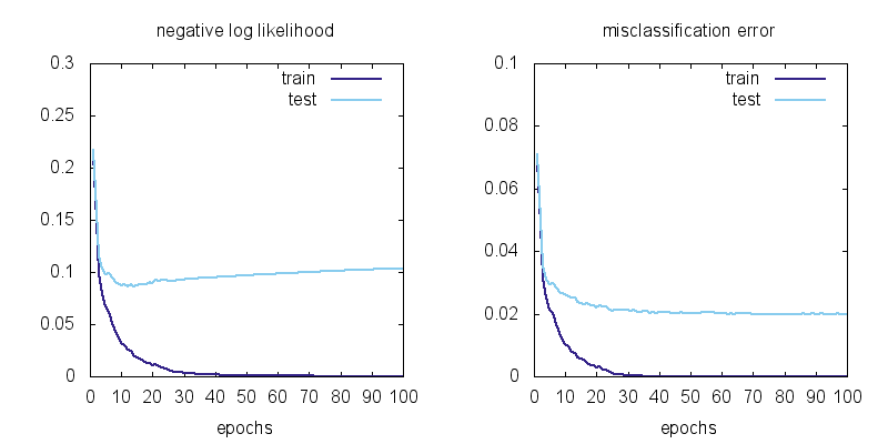
Here are the learning curves for the linear model mnist_softmax
plotted at the same scale for comparison:
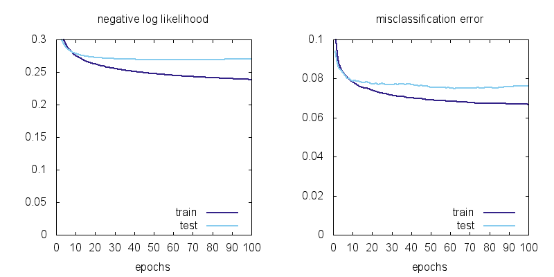
We can observe a few things: using MLP instead of a linear model brings the training error from 6.7% to 0 and the test error from 7.5% to 2.0%. There is still overfitting: the test error is not as good as the training error, but the model has no problem classifying the training data (all 60,000 examples) perfectly!
Types of nonlinearities (activation functions)
The functions we throw between linear layers to break the linearity are called nonlinearities or activation functions. Here are some activation functions that have been used as nonlinearities:
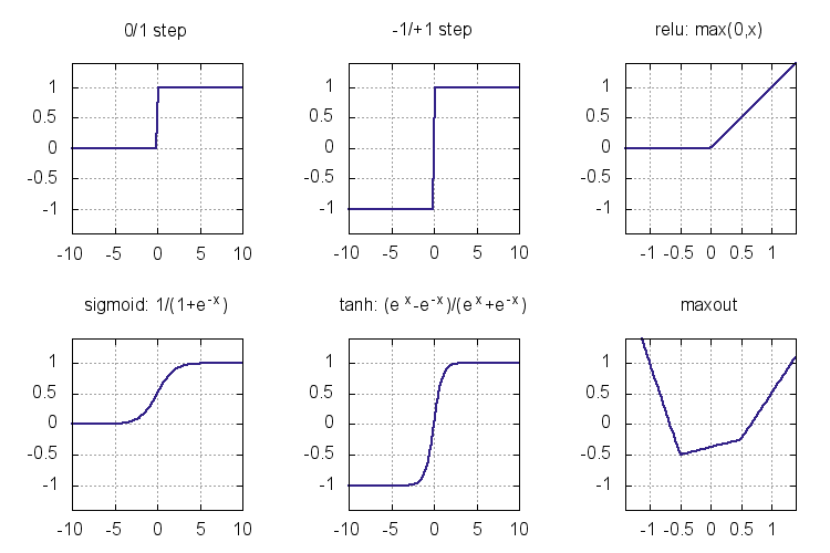
The step functions were the earliest activation functions used in the
perceptrons of 1950s. Unfortunately they do not give a useful
derivative that can be used for training a multilayer model. Sigmoid
and tanh (sigm and tanh in Knet) became popular in 1980s as
smooth approximations to the step functions and allowed the
application of the backpropagation algorithm. Modern activation
functions like relu and maxout are piecewise linear. They are
computationally inexpensive (no exponentials), and perform well in
practice. We are going to use relu in most of our models. Here is
the backward passes for sigmoid, tanh, and relu:
| function | forward | backward |
|---|---|---|
| sigmoid | \(y = \frac{1}{1+e^{-x}}\) | \(\nabla_x J = y\,(1-y) \nabla_y J\) |
| tanh | \(y = \frac{e^x-e^{-x}}{e^x+e^{-x}}\) | \(\nabla_x J = (1+y)(1-y) \nabla_y J\) |
| relu | \(y = \max(0,x)\) | \(\nabla_x J = [ y \geq 0 ] \nabla_y J\) |
See (Karpathy, 2016, Ch 1) for more on activation functions and MLP architecture.
Representational power
You might be wondering whether relu had any special properties or
would any of the other nonlinearities be sufficient. Another question
is whether there are functions multilayer perceptrons cannot represent
and if so whether adding more layers or different types of functions
would increase their representational power. The short answer is that
a two layer model can approximate any function if the hidden layer is
large enough, and can do so with any of the nonlinearities introduced
in the last section. Multilayer perceptrons are universal function
approximators!
We said that a two-layer MLP is a universal function approximator given enough hidden units. This brings up the questions of efficiency: how many hidden units / parameters does one need to approximate a given function and whether the number of units depends on the number of hidden layers. The efficiency is important both computationally and statistically: models with fewer parameters can be evaluated faster, and can learn from fewer examples (ref?). It turns out there are functions whose representations are exponentially more expensive in a shallow network compared to a deeper network (see (Nielsen, 2016, Ch 5) for a discussion). Recent winners of image recognition contests use networks with dozens of convolutional layers. The advantage of deeper MLPs is empirically less clear, but you should experiment with the number of units and layers using a development set when starting a new problem.
Please see (Nielsen, 2016, Ch 4) for an intuitive explanation of the universality result and (Bengio et al. 2016, Ch 6.4) for a more in depth discussion and references.
Matrix vs Neuron Pictures
So far we have introduced multilayer perceptrons (aka artificial neural networks) using matrix operations. You may be wondering why people call them neural networks and be confused by terms like layers and units. In this section we will give the correspondence between the matrix view and the neuron view. Here is a schematic of a biological neuron (figures from (Karpathy, 2016, Ch 1)):
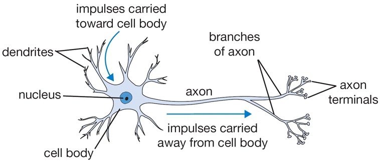
A biological neuron is a complex organism supporting thousands of chemical reactions simultaneously under the regulation of thousands of genes, communicating with other neurons through electrical and chemical pathways involving dozens of different types of neurotransmitter molecules. We assume (do not know for sure) that the main mechanism of communication between neurons is electrical spike trains that travel from the axon of the source neuron, through connections called synapses, into dendrites of target neurons. We simplify this picture further representing the strength of the spikes and the connections with simple numbers to arrive at this cartoon model:
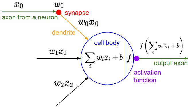
This model is called an artificial neuron, a perceptron, or simply a unit in neural network literature. We know it as the softmax classifier.
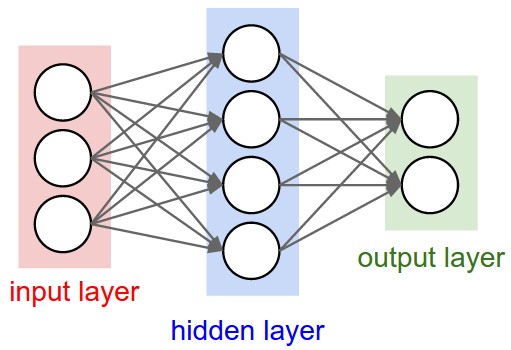
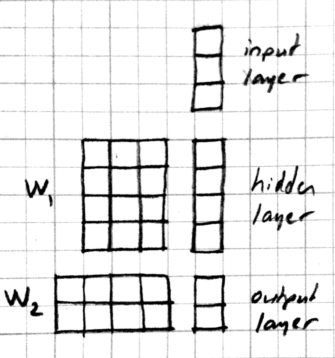
When a number of these units are connected in layers, we get a multilayer perceptron. When counting layers, we ignore the input layer. So the softmax classifier can be considered a one layer neural network. Here is a neural network picture and the corresponding matrix picture for a two layer model:
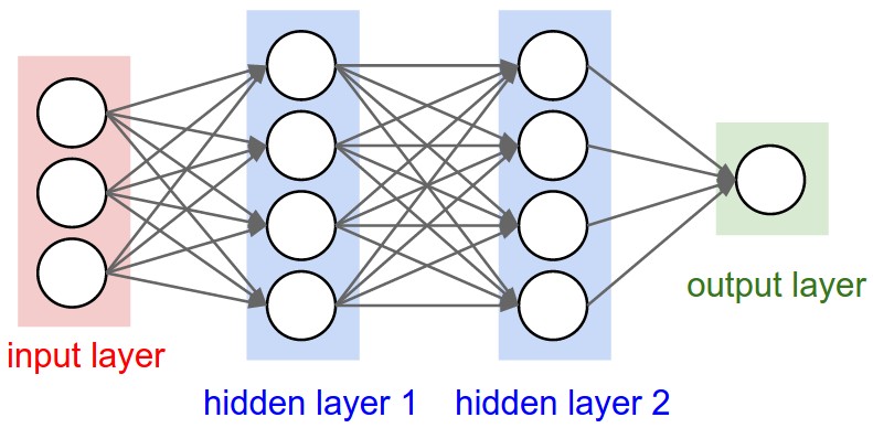
Here is a neural network picture and the corresponding matrix picture for a three layer model:
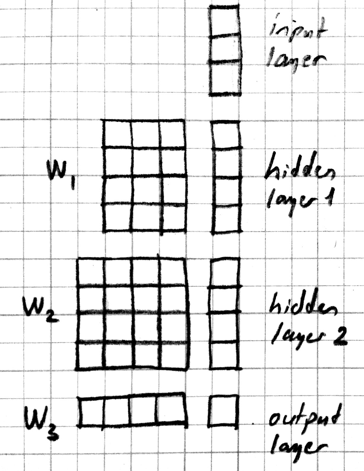
We can use the following elementwise notation for the neural network picture (e.g. similar to the one used in UFLDL):
Here \(x_i^{(l)}\) refers to the activation of the \(i\) th unit in \(l\) th layer. We are counting the input as the 0’th layer. \(f\) is the activation function, \(b_i^{(l)}\) is the bias term. \(w_{ij}^{(l)}\) is the weight connecting unit \(j\) from layer \(l-1\) to unit \(i\) from layer \(l\). The corresponding matrix notation is:
Programming Example
In this section we introduce several Knet features that make it easier to define complex models. As our working example, we will go through several attempts to define a 3-layer MLP. Here is our first attempt:
@knet function mlp3a(x0)
    w1 = par(init=Gaussian(0,0.001), dims=(100,28*28))
    b1 = par(init=Constant(0), dims=(100,1))
    x1 = relu(w1 * x0 + b1)
    w2 = par(init=Gaussian(0,0.001), dims=(100,100))
    b2 = par(init=Constant(0), dims=(100,1))
    x2 = relu(w2 * x1 + b2)
    w3 = par(init=Gaussian(0,0.001), dims=(10,100))
    b3 = par(init=Constant(0), dims=(10,1))
    return soft(w3 * x2 + b3)
end
We can identify several bad software engineering practices in this definition:
- It contains a lot of repetition.
- It has a number of hardcoded parameters.
The key to controlling complexity in computer languages is abstraction. Abstraction is the ability to name compound structures built from primitive parts, so they too can be used as primitives. In Knet we do this by using @knet functions not as models, but as new operators inside other @knet functions.
Defining new operators
We could make the definition of mlp3 more compact by defining @knet functions for its layers:
@knet function mlp3b(x0)
    x1 = relu_layer1(x0)
    x2 = relu_layer2(x1)
    return soft_layer3(x2)
end

@knet function relu_layer1(x)
    w = par(init=Gaussian(0,0.001), dims=(100,28*28))
    b = par(init=Constant(0), dims=(100,1))
    return relu(w * x + b)
end

@knet function relu_layer2(x)
    w = par(init=Gaussian(0,0.001), dims=(100,100))
    b = par(init=Constant(0), dims=(100,1))
    return relu(w * x + b)
end

@knet function soft_layer3(x)
    w = par(init=Gaussian(0,0.001), dims=(10,100))
    b = par(init=Constant(0), dims=(10,1))
    return soft(w * x + b)
end
This may make the definition of mlp3b a bit more readable. But it
does not reduce the overall length of the program. The helper @knet
functions like relu_layer1 contain hardcoded parameters like
dims and are not reusable.
Using keyword arguments
We can make @knet functions more reusable by using keyword arguments
that make them configurable. Here is a more compact definition of
mlp3 using a single helper @knet function, wbf (mnemonic for
\(f(w*x+b)\)):
@knet function mlp3c(x0)
    x1 = wbf(x0; f=:relu, inputs=28*28, outputs=100)
    x2 = wbf(x1; f=:relu, inputs=100, outputs=100)
    return wbf(x2; f=:soft, inputs=100, outputs=10)
end

@knet function wbf(x; f=:relu, inputs=0, outputs=0, winit=Gaussian(0,0.001), binit=Constant(0))
    w = par(init=winit, dims=(outputs,inputs))
    b = par(init=binit, dims=(outputs,1))
    return f(w * x + b)
end
Size inference
Knet can infer the size of an array based on the operations and other
arrays it interacts with. In particular, when forw(f,x) is called
Knet uses the size of the input x to figure out what size
intermediate arrays to allocate when computing f. This allows us
to define generic models and operators that work on inputs of any
size. We still need to specify the number of outputs, but the number
of inputs can be left unspecified. By convention 0 represents
“unspecified” when declaring dimensions. Here is a more generic
version of mlp3 that will work on images of any size:
@knet function mlp3d(x0)
    x1 = wbf(x0; f=:relu, out=100)
    x2 = wbf(x1; f=:relu, out=100)
    return wbf(x2; f=:soft, out=10)
end

@knet function wbf(x; f=:relu, out=0, winit=Gaussian(0,0.001), binit=Constant(0))
    w = par(init=winit, dims=(out,0))
    b = par(init=binit, dims=(out,1))
    return f(w * x + b)
end
Higher-order operators
Higher-order operators are ones that take other operators as
arguments. We have already seen an example: wbf takes an operator
f as one of its keyword arguments. A useful higher-order operator
for multi-layer models is repeat, which repeats a given operator
specified by frepeat configured by other keyword arguments a given
number of times specified by nrepeat. Here is a definition of
mlp3 using repeat:
@knet function mlp3e(x; o...)
    h = repeat(x; frepeat=:wbf, nrepeat=2, f=:relu, out=100, o...)
    return wbf(h; f=:soft, out=10)
end

@knet function wbf(x; f=:relu, out=0, winit=Gaussian(0,0.001), binit=Constant(0))
    w = par(init=winit, dims=(out,0))
    b = par(init=binit, dims=(out,1))
    return f(w * x + b)
end
In this example repeat saved us a single line, but the difference
can be more significant in deeper models.
Built-in operators
In addition to primitive operators like relu, many compound
operators such as wbf are already defined in Knet to make it
easier to define complex models. Please see the tables of
primitive operators and compound
operators for a summary and kfun.jl for exact
definitions.